A colorful scatter plot
Learn how to create a colorful scatter plot using DataPicta.
This tutorial guides you through creating a scatterplot chart using the DataPicta application. You will learn how to load sample data, change the values for the horizontal and vertical axes and how to add a third color axis.
Go to app.datapicta.com to open the DataPicta application.
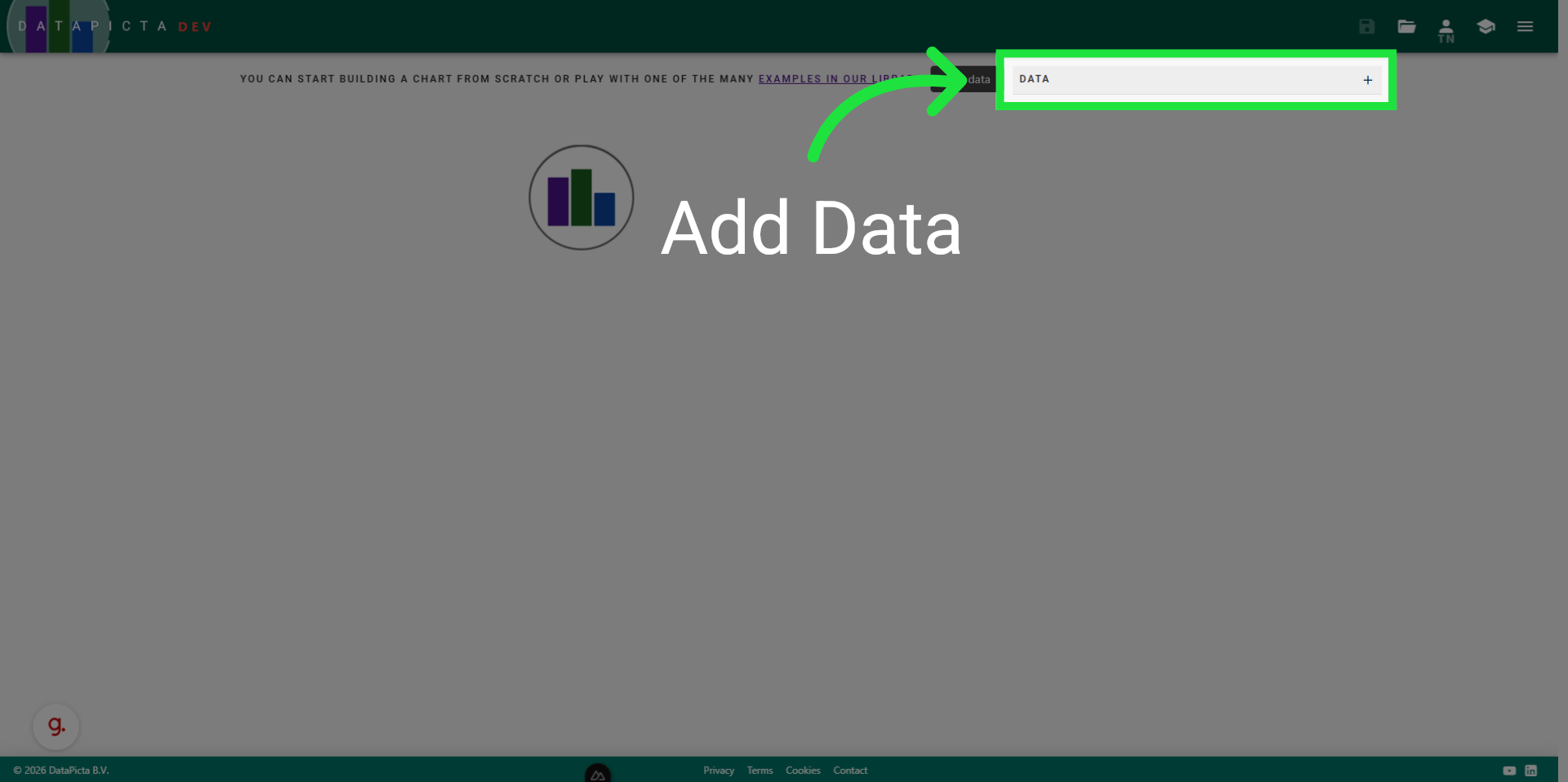
1. Add Data
Every chart creation begins with a good dataset. To add data click on 'Add data' here.
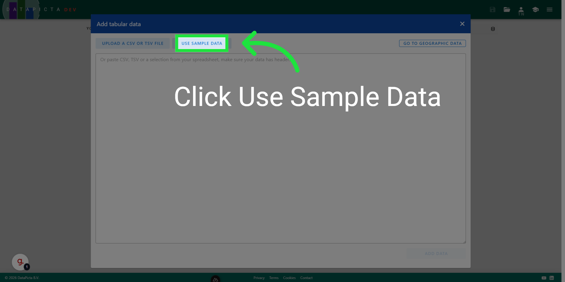
2. Use Sample Data
For this tutorial we will use one of the many sample datasets DataPicta offers. Click on 'Use Sample Data'.
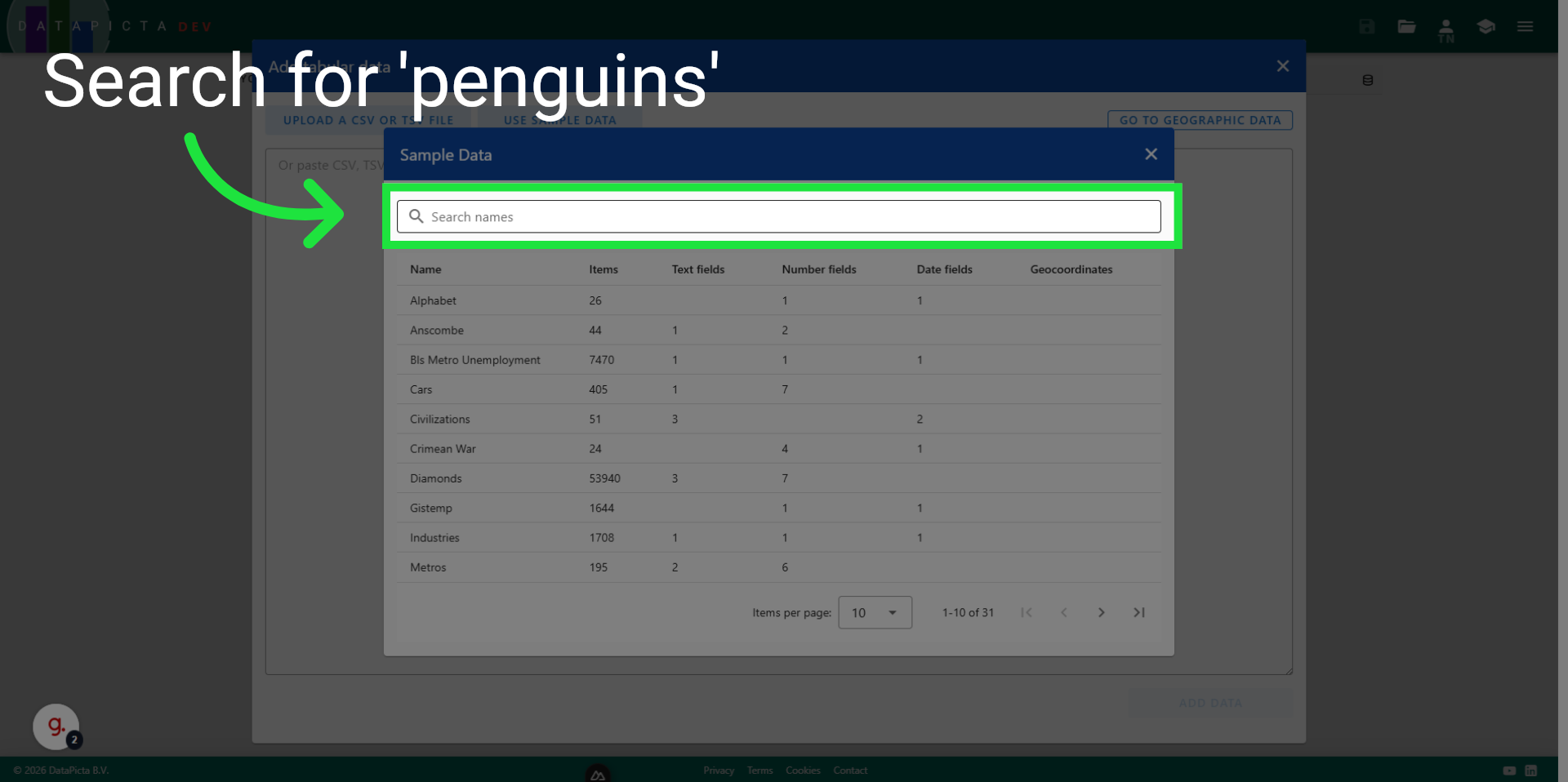
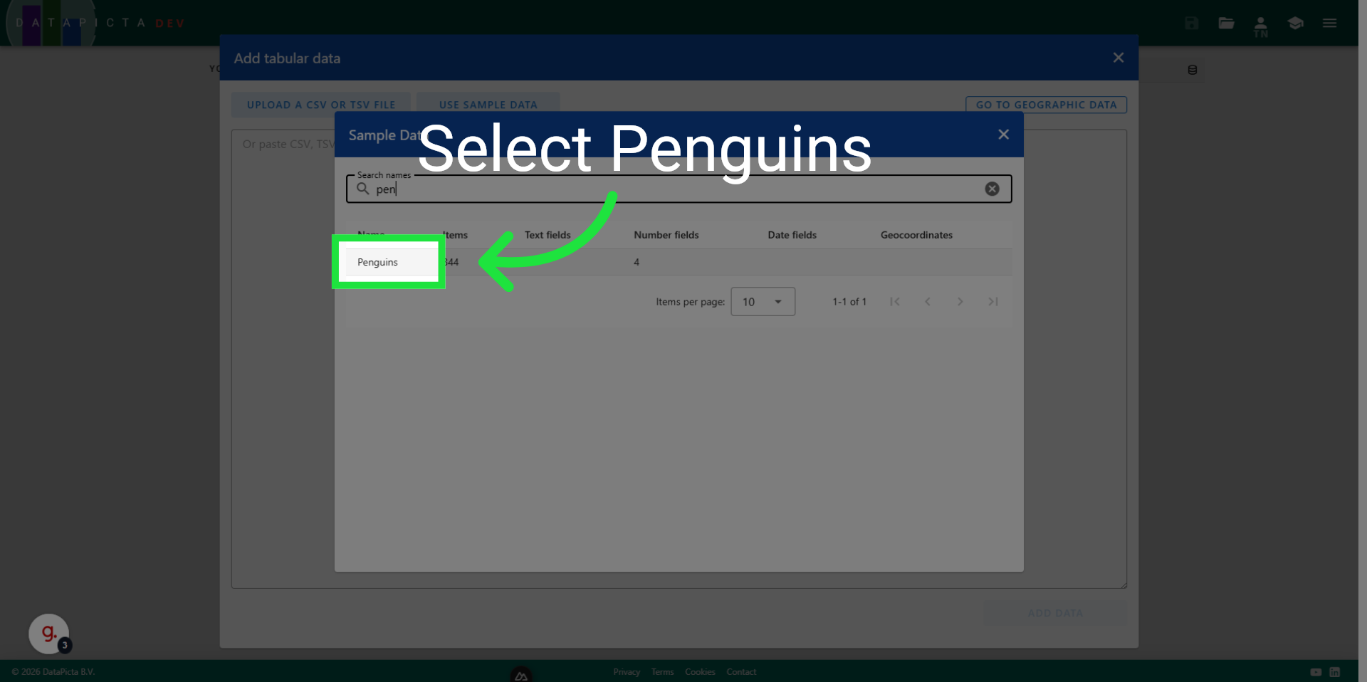
3. Search penguins
Click 'Search names' to begin filtering the dataset by name. We will be using the 'Penguins' dataset.
4. Click Penguins
Click 'Penguins' to load the penguins dataset.
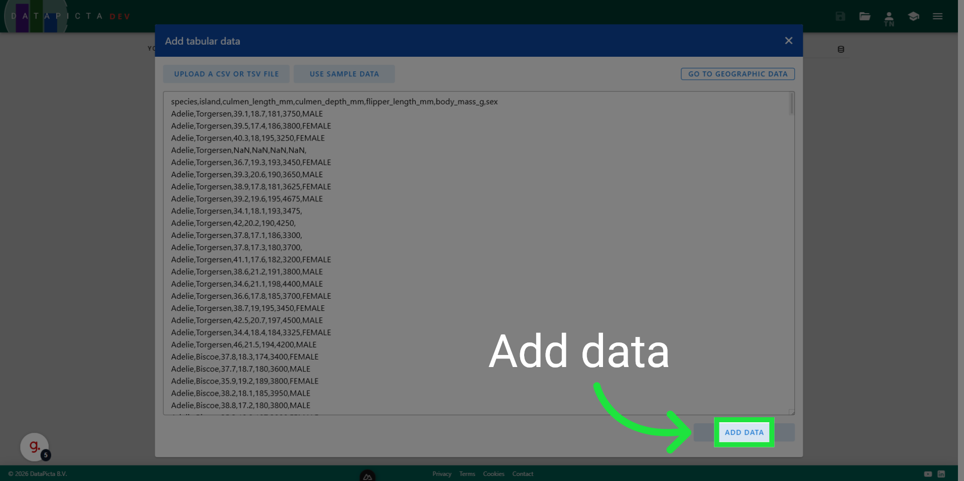
5. Add Data to Visualization
Click 'Add data'' to include the selected dataset in your visualization.
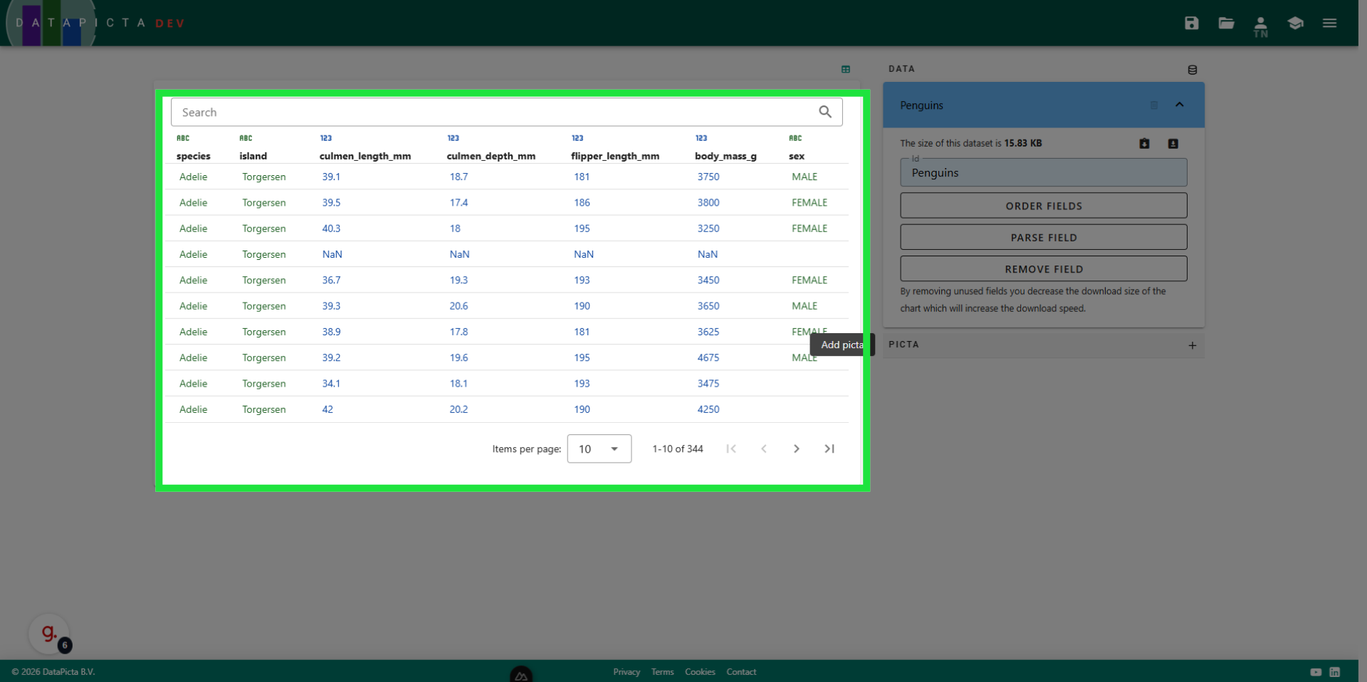
6. View Data
This dataset features penguins and includes four measurements across three species. To create scatter plots, you require a minimum of two measurements, meaning two columns of numerical data. This dataset is perfect for a scatter plot.
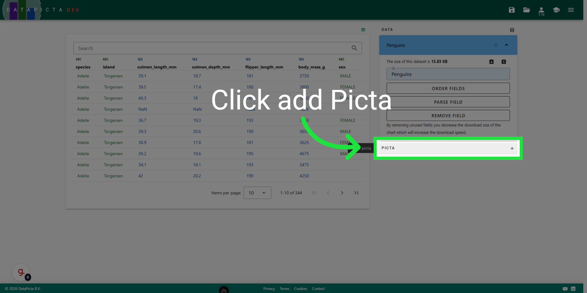
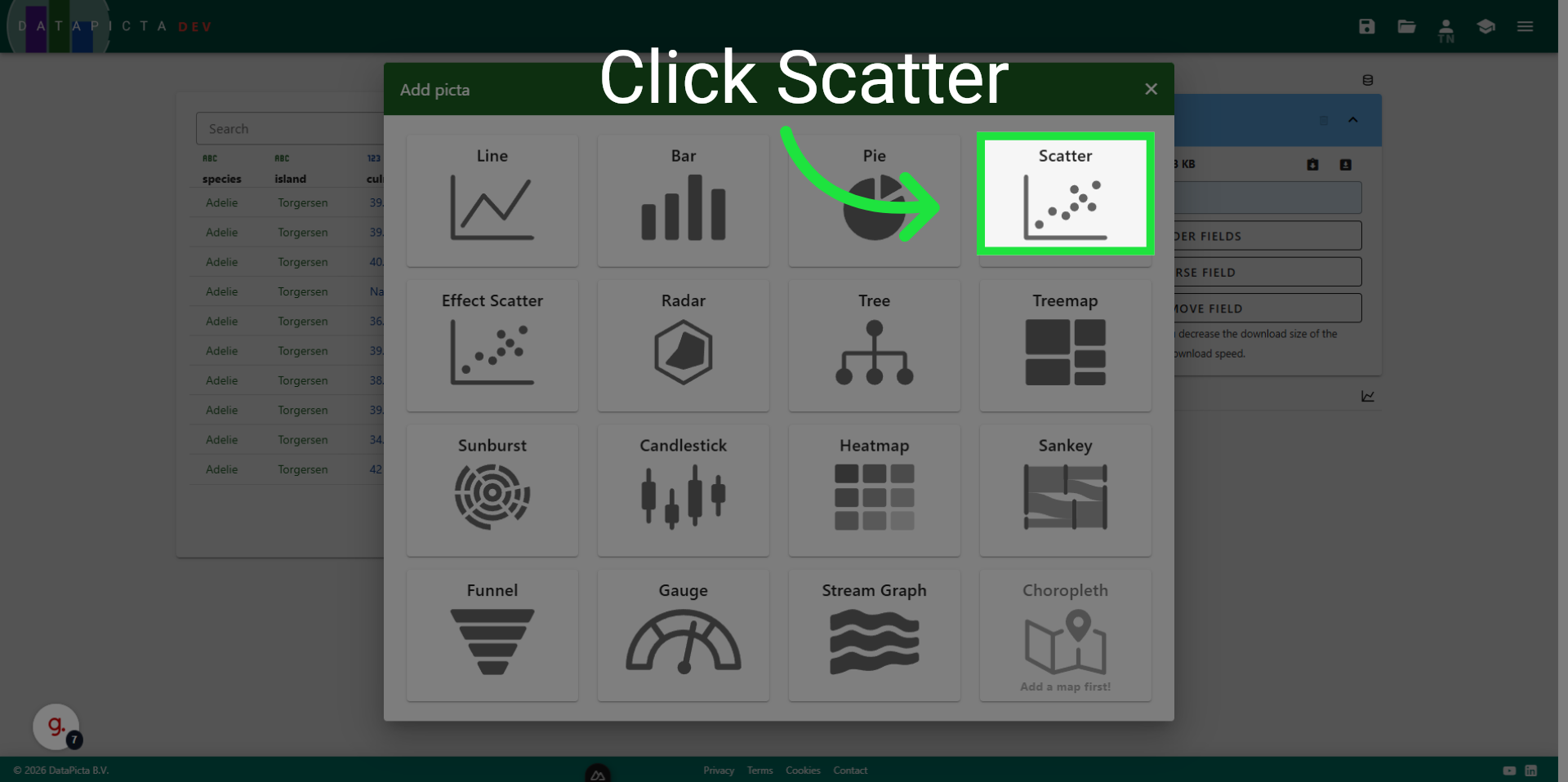
7. Add Picta
Every visualization needs a picta, such as bar, line, or scatter. Click here to add a picta.
8. Choose Scatter Picta
Choose the scatter picta.
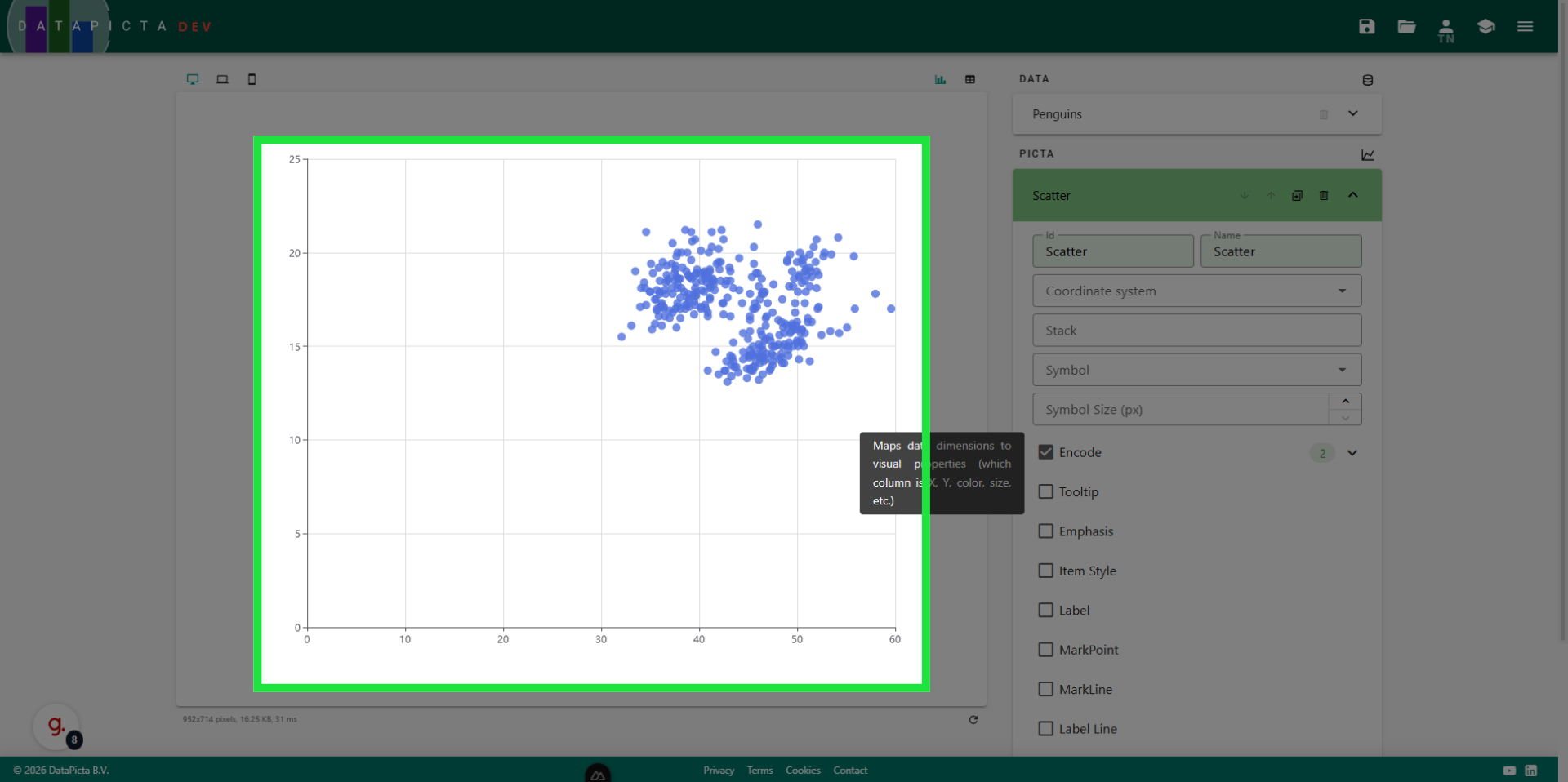
9. View Scatter Picta
When a picta is selected, it automatically assigns data fields to the axes. For the scatter picta, it chooses the first two numerical fields.
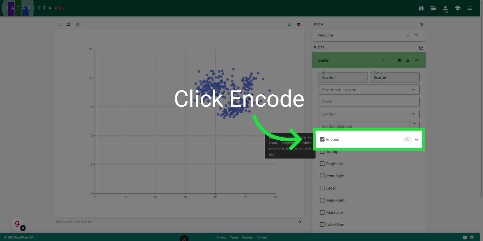
10. Select Data Binding
But we will map the axes to two different numerical fields. To do this, click 'Data Binding'.
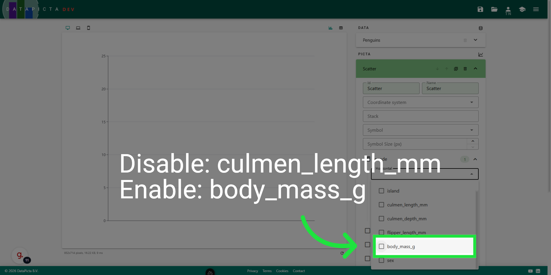
11. Edit Horizontal Axis
Disable the 'Culmen length' field and enable the 'Body mass' field for the horizontal axis.
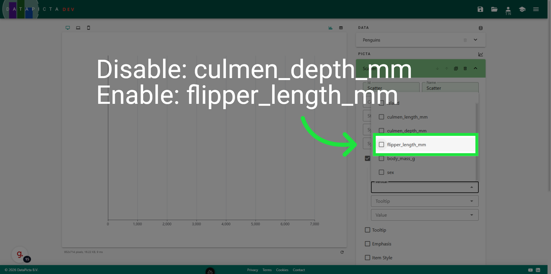
12. Edit Vertical Axis
Disable the 'Culmen depth' field and enable the 'Flipper length' field for the vertical axis.
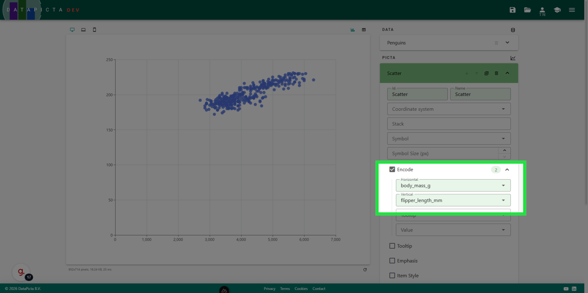
13. Review Settings
Please confirm that you have selected 'body mass' and 'flipper length.' While it is possible to assign multiple fields to a single axis, doing so often reduces the readability of the visualization.
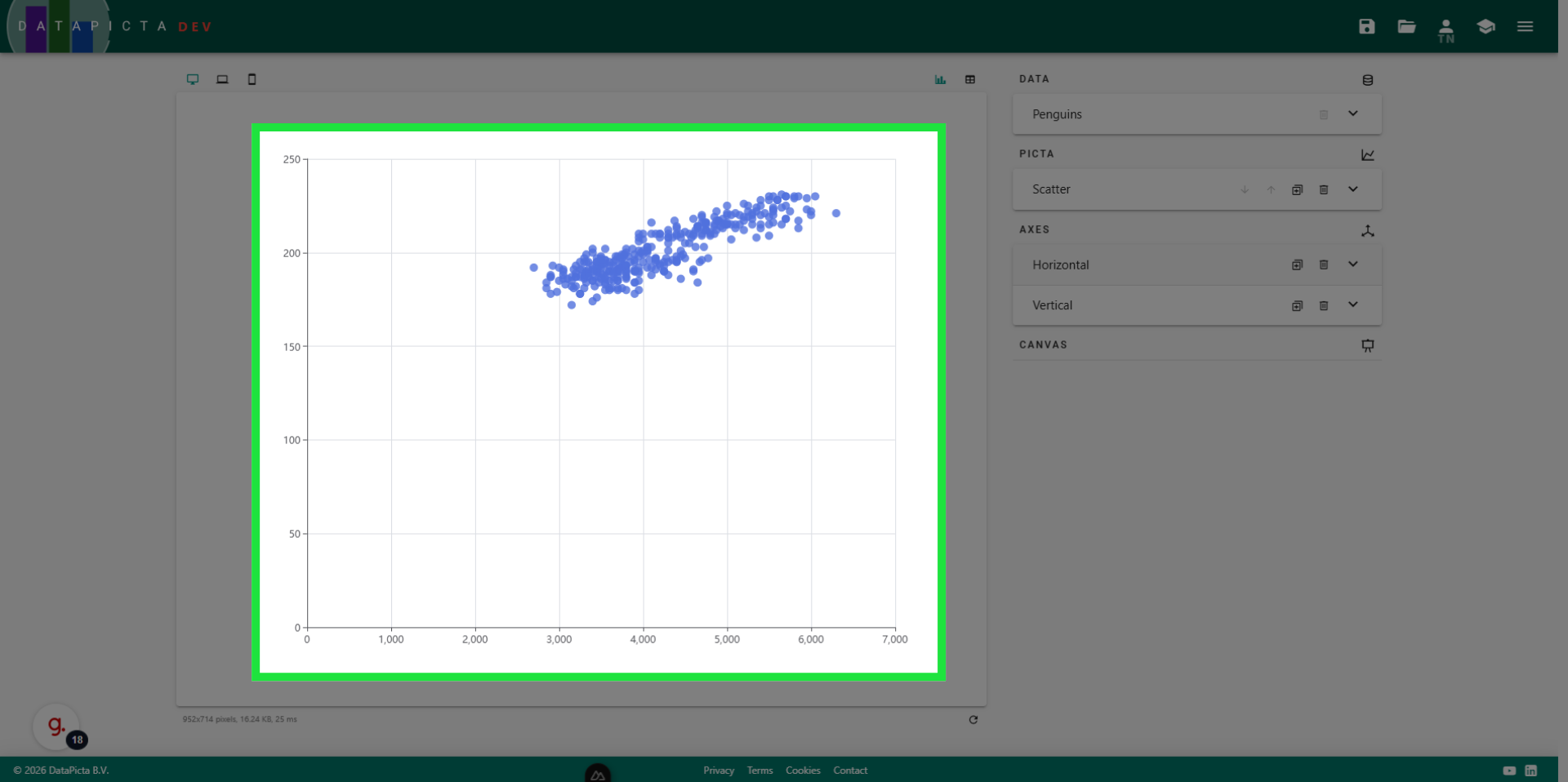
14. View Result in Chart
The visualization has changed due to the newly assigned fields on the axis. We will now implement further enhancements to make the visualization more appealing, starting with improvements to the axes.
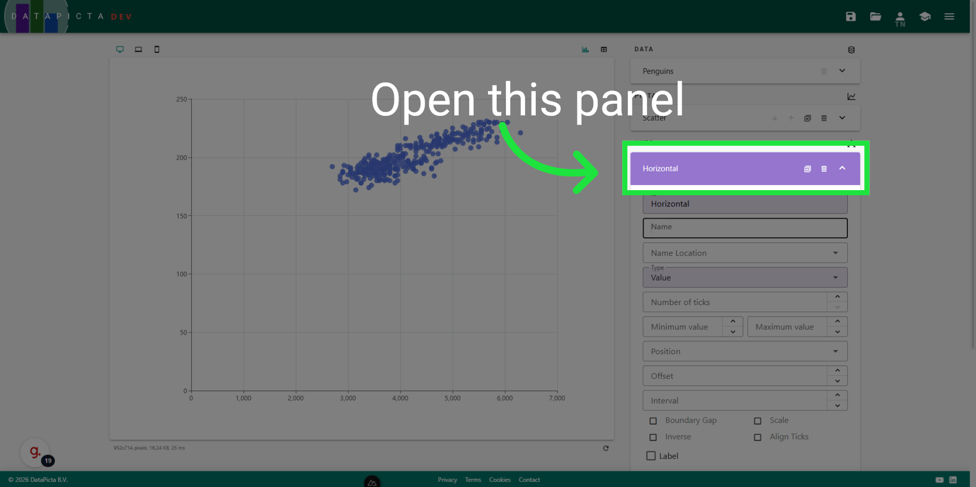
15. Open Horizontal Panel
Open the horizontal panel to adjust the horizontal axis.
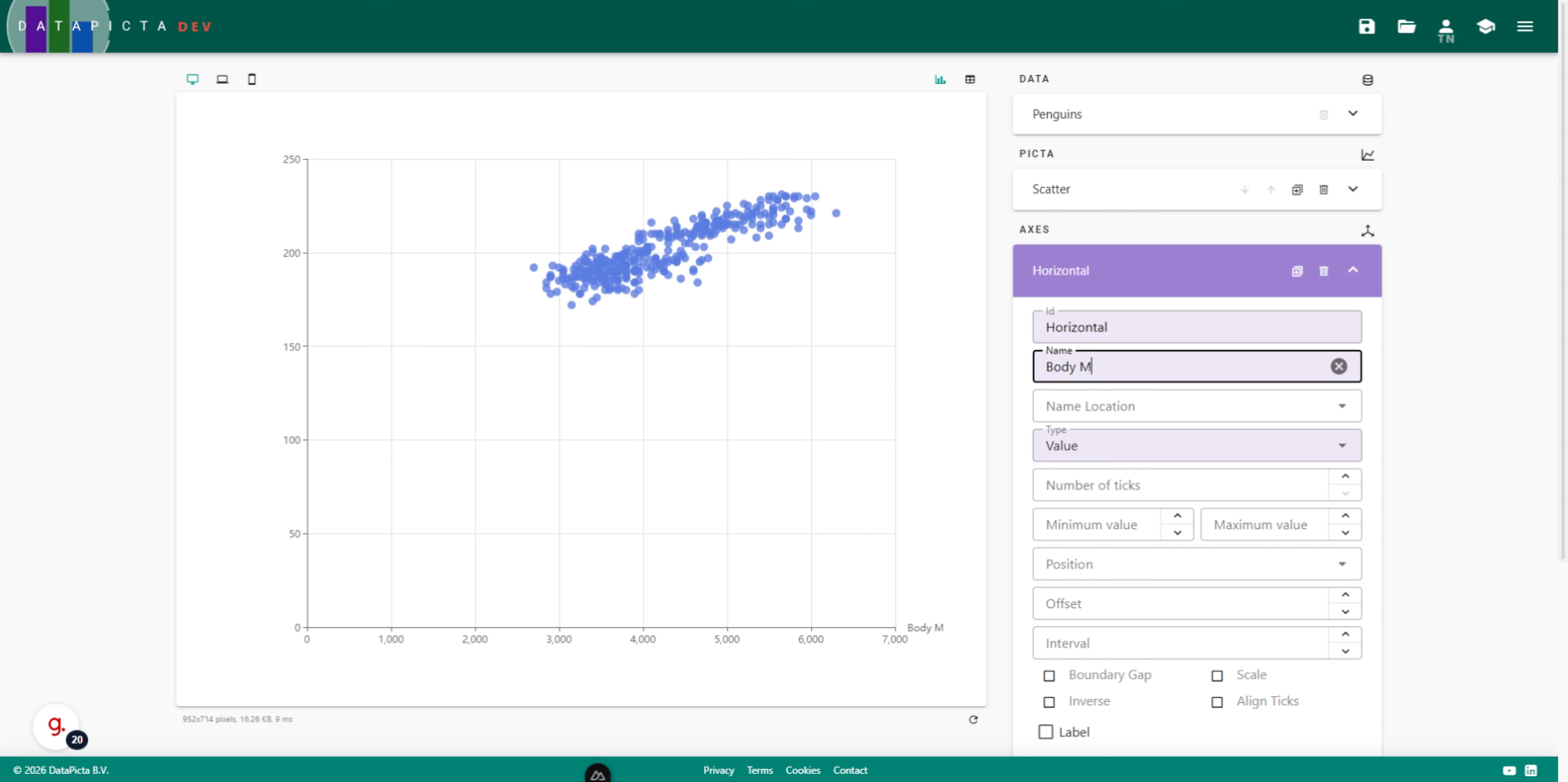
16. Set Name
In the name field type 'Body Mass'' to add a name for this axis.
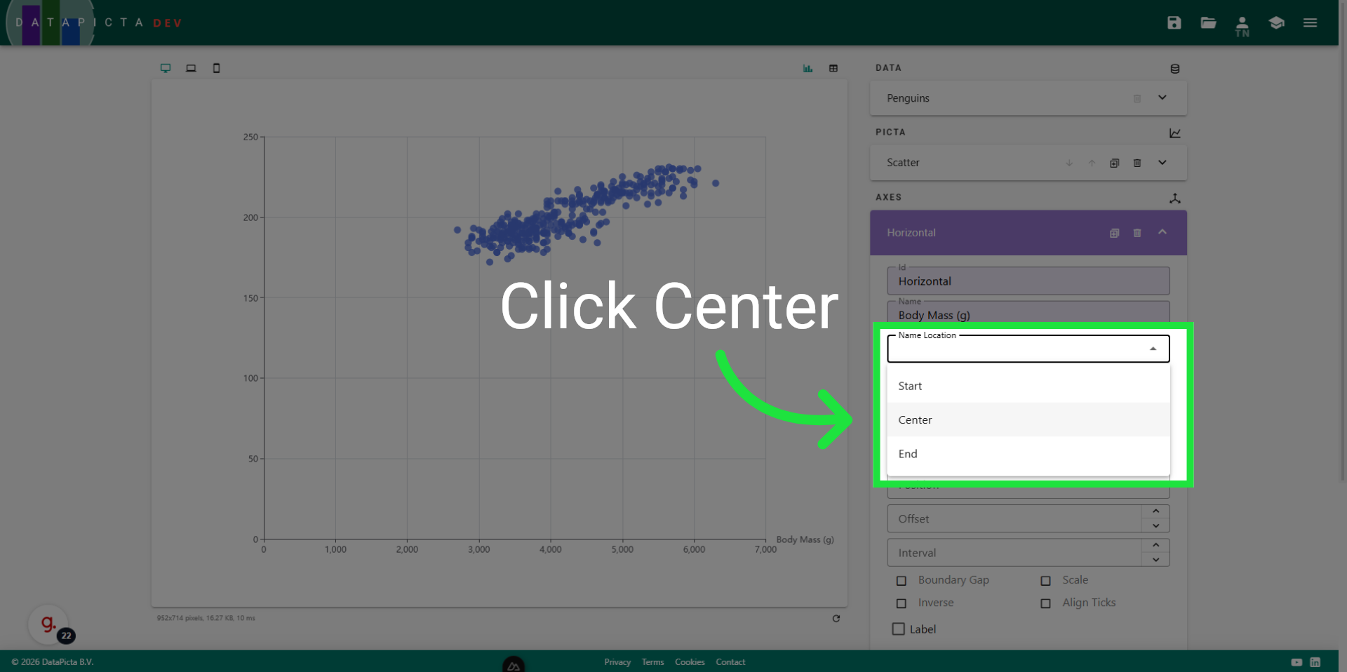
17. Center Name
Click 'center' in the 'name location' field to position the name at the center of the chart.
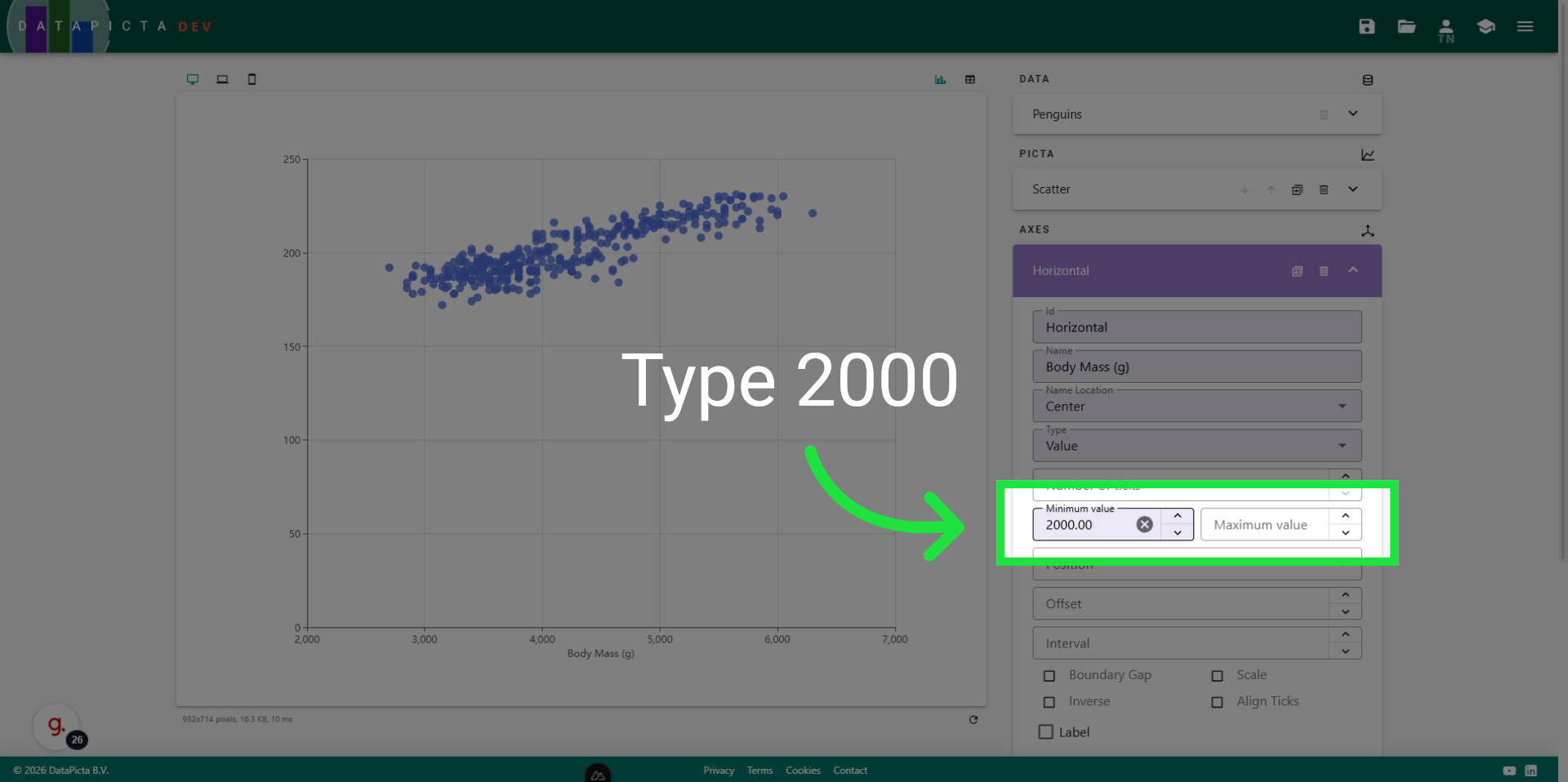
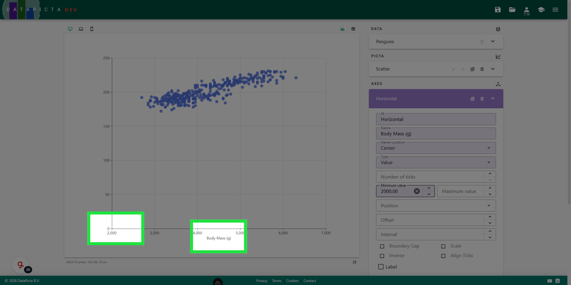
18. Set Minimum Value
By default, an axis begins at zero. To minimize white space in the chart, we adjust the starting point. For 'minimum value', enter '2000'.
19. Confirm Axis Settings
Please confirm that you have adjusted the horizontal axis as follows.
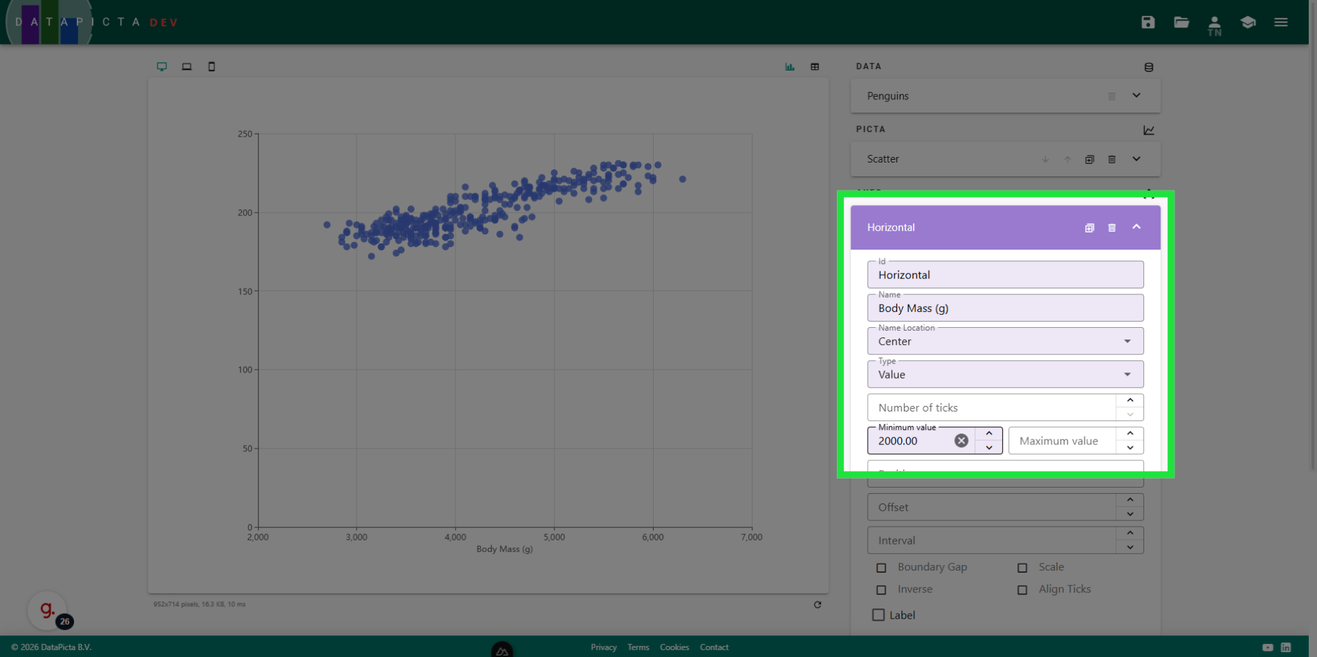
20. View Result
The changes are applied immediately.
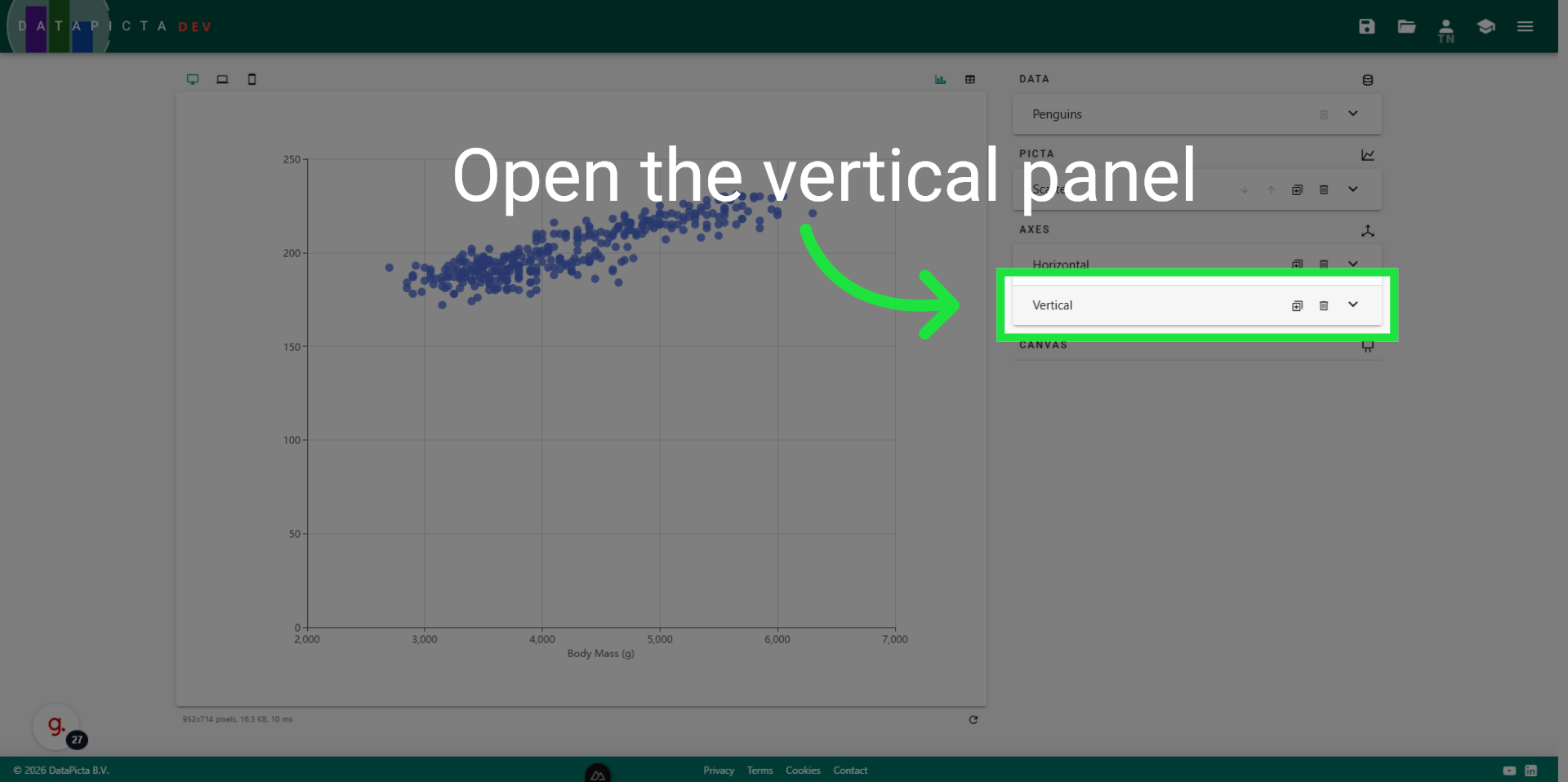
21. Open Vertical Panel
We will implement similar adjustments to the vertical axis. Please close the horizontal panel and open the vertical panel.
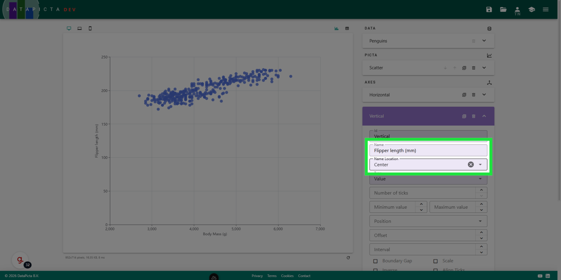
22. Edit Name and Location
Change the name of the vertical axis to 'Flipper length' and center its location.
23. Set Minimum Value
Type '160' for the minimum value.
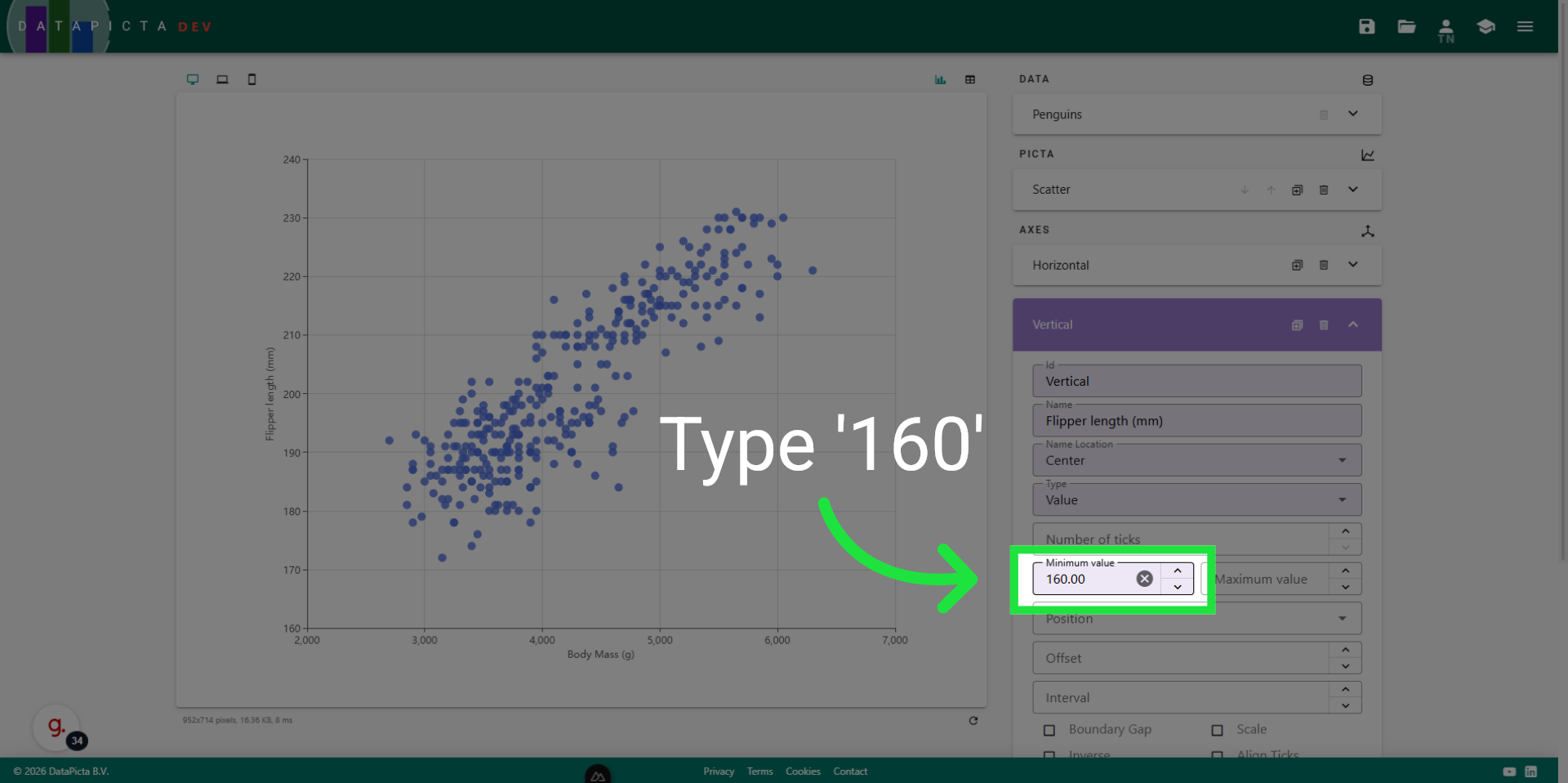
24. View Result
The scatter plot looks significantly better now. We can enhance this chart further by coloring the dots based on the penguin species they represent.
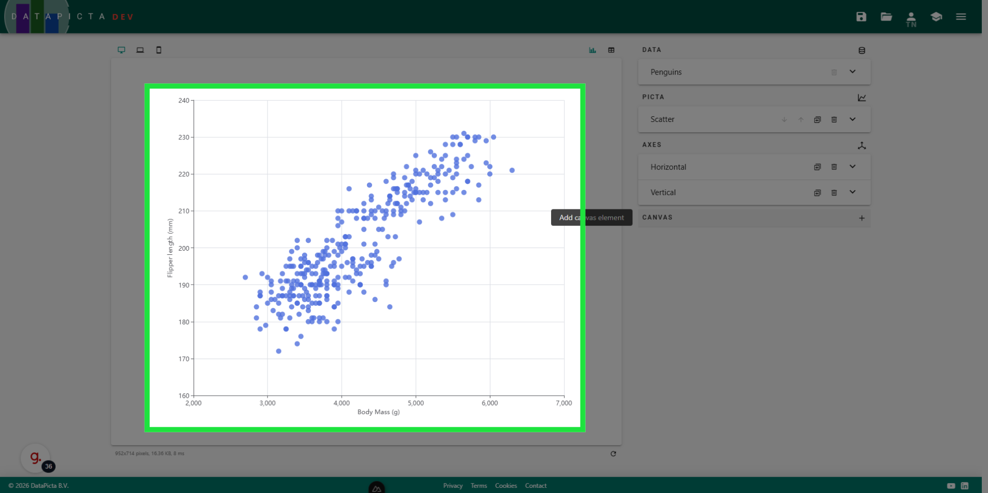
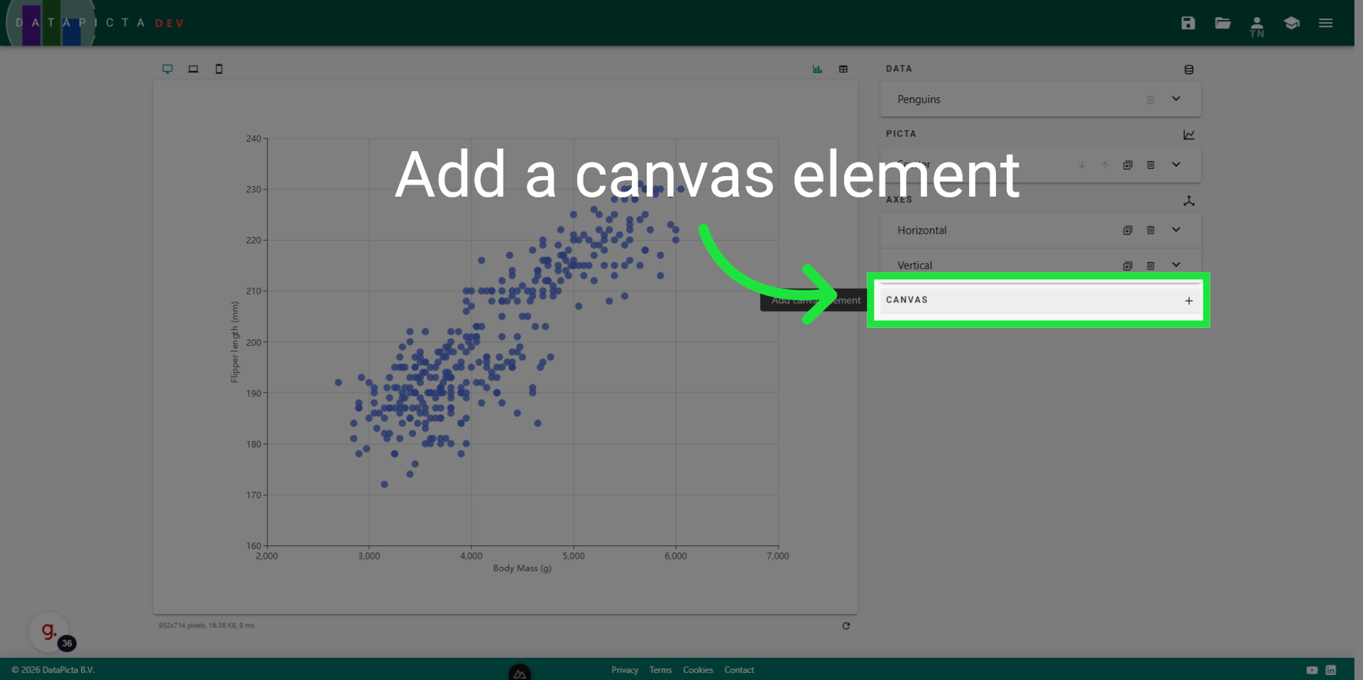
25. Add Canvas Element
Click here to add a canvas element to this chart.
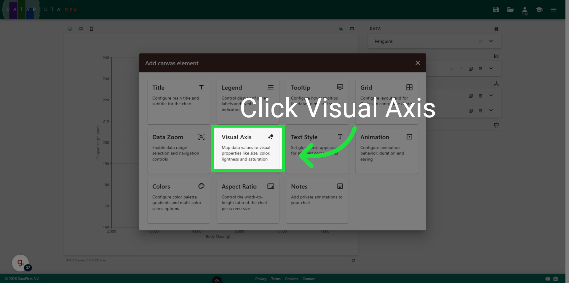
26. Choose Visual Axis
A visual axis is an axis represented by color or size.
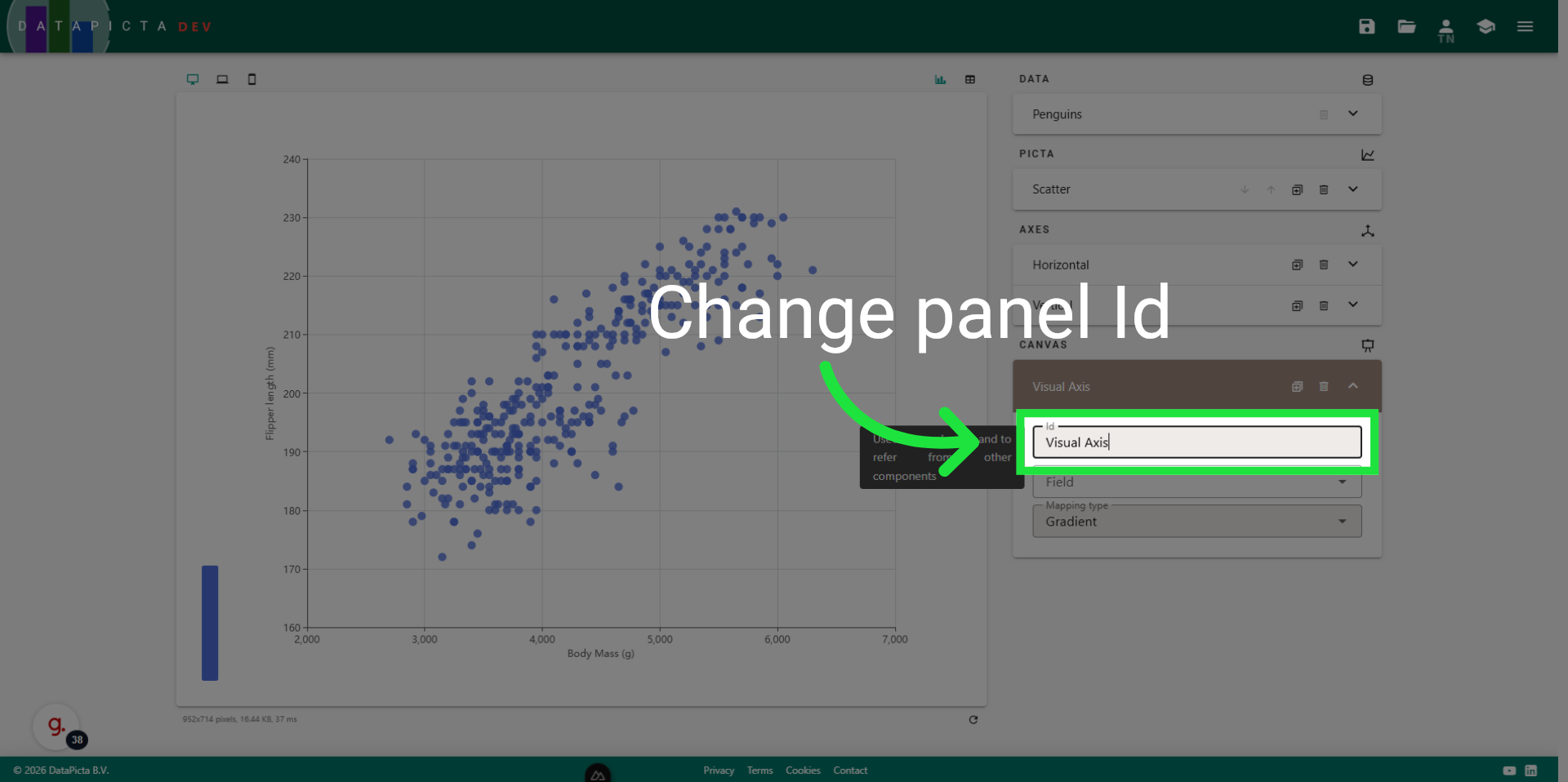
27. Edit Id
You can rename the Id of the visual axis. While this does not affect the chart itself, it updates the panel name to something more understandable. We renamed it to 'Species color'.
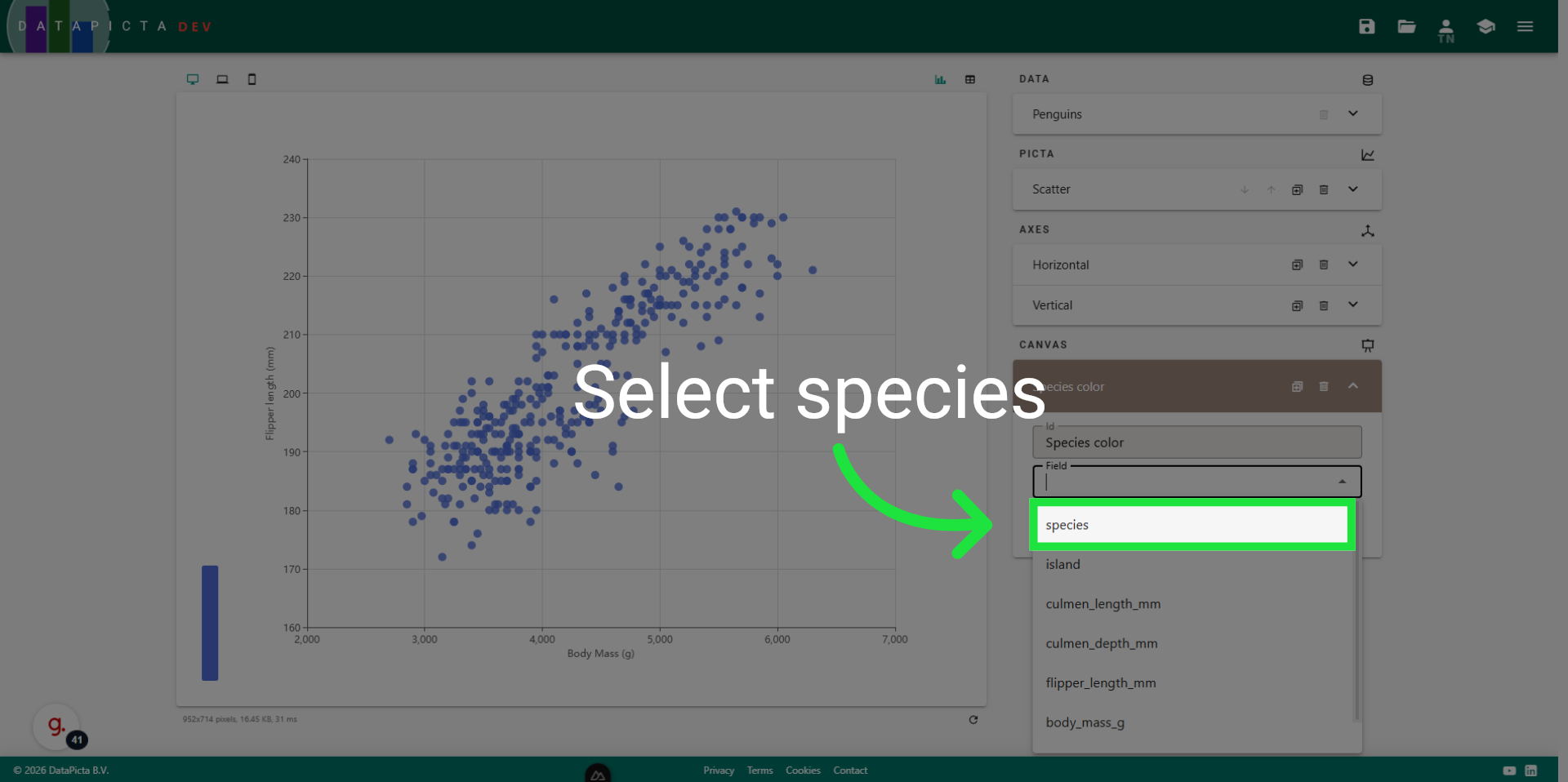
28. Choose Species Field
We will utilize the 'Species' field for coloring. The dataset includes three distinct species of penguins.
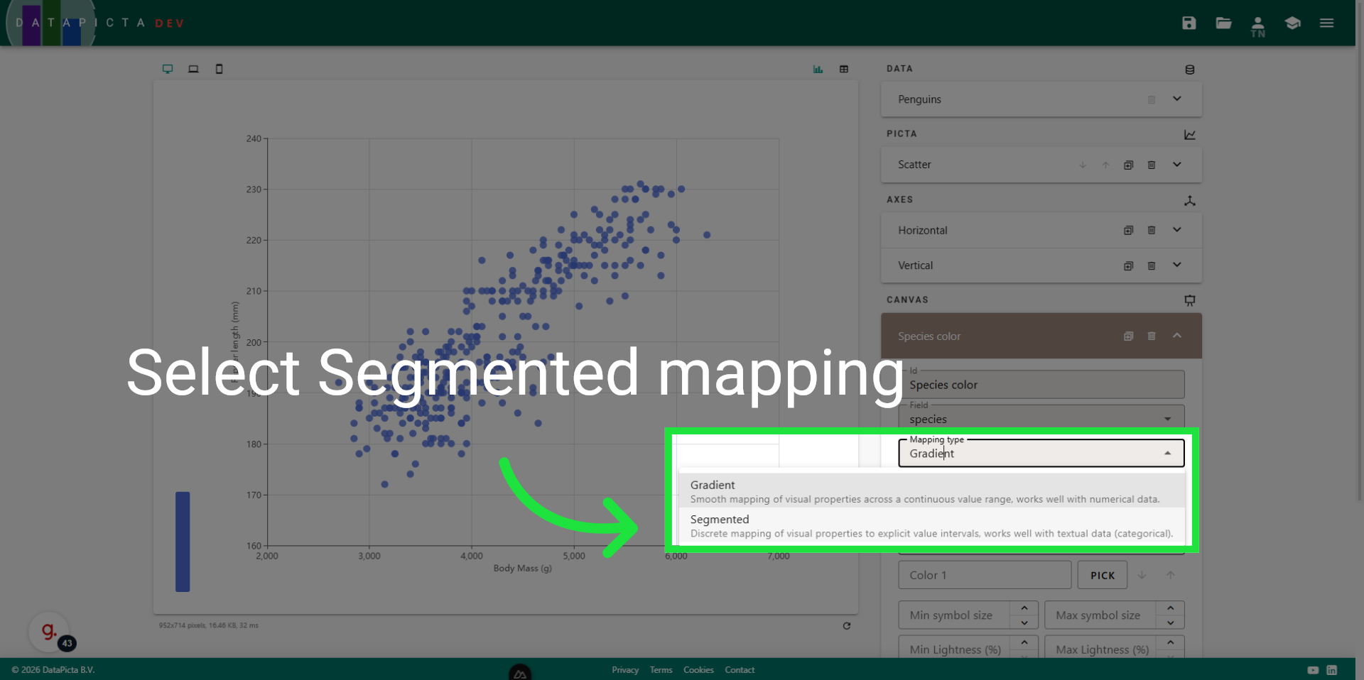
29. Select Segmented
Since 'species' has three distinct values and no intermediate measurements, we will use three separate colors. Therefore, click 'Segmented' as the mapping type.
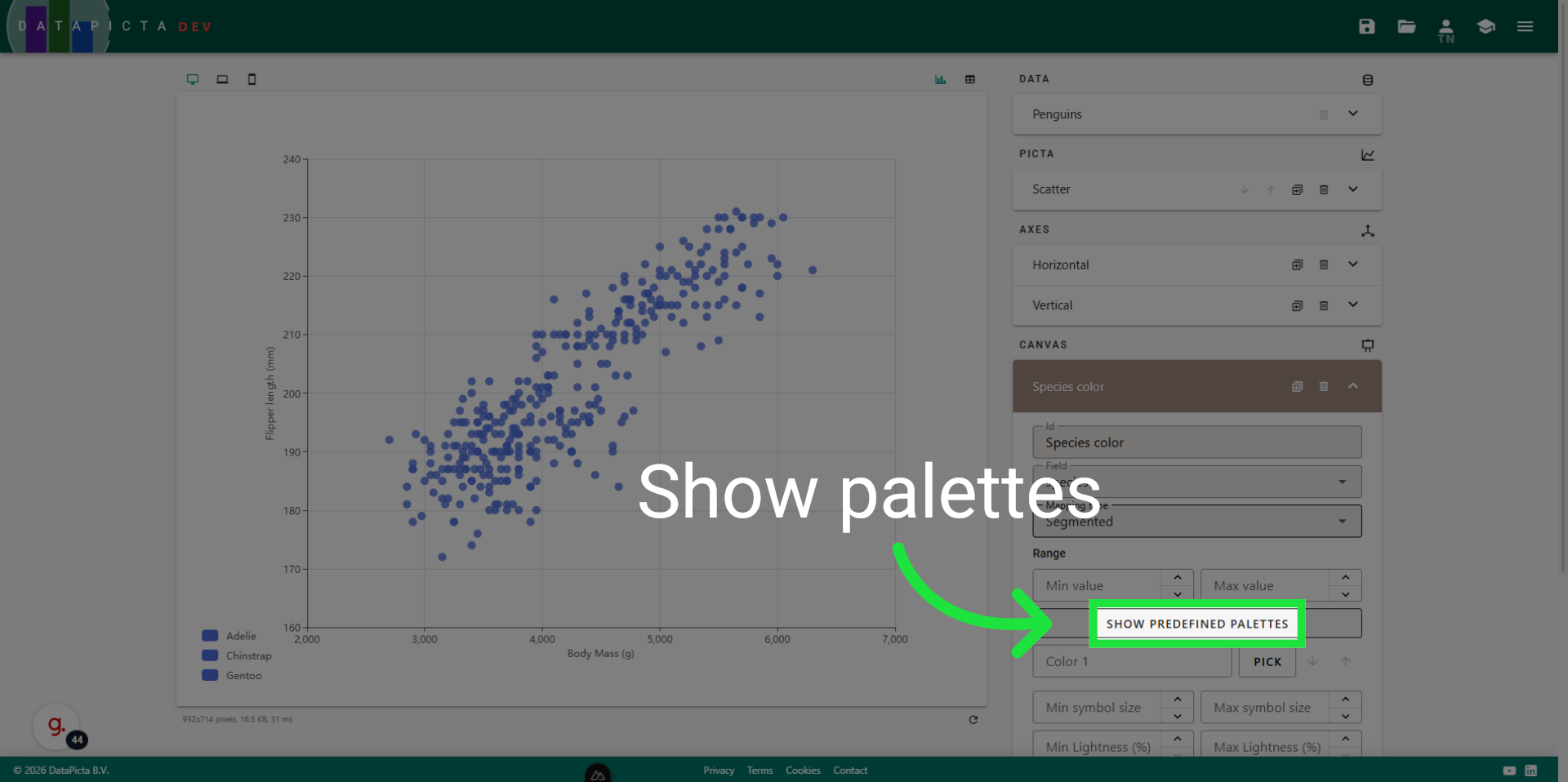
30. Show Color Palettes
You can manually define up to three colors or choose from one of the predefined color palettes. We prefer the simpler option and click 'Show predefined palettes'.
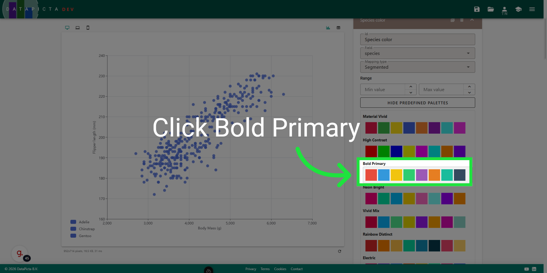
31. Pick a Palette
We have selected the 'Bold Primary' palette; however, you are welcome to choose your own.
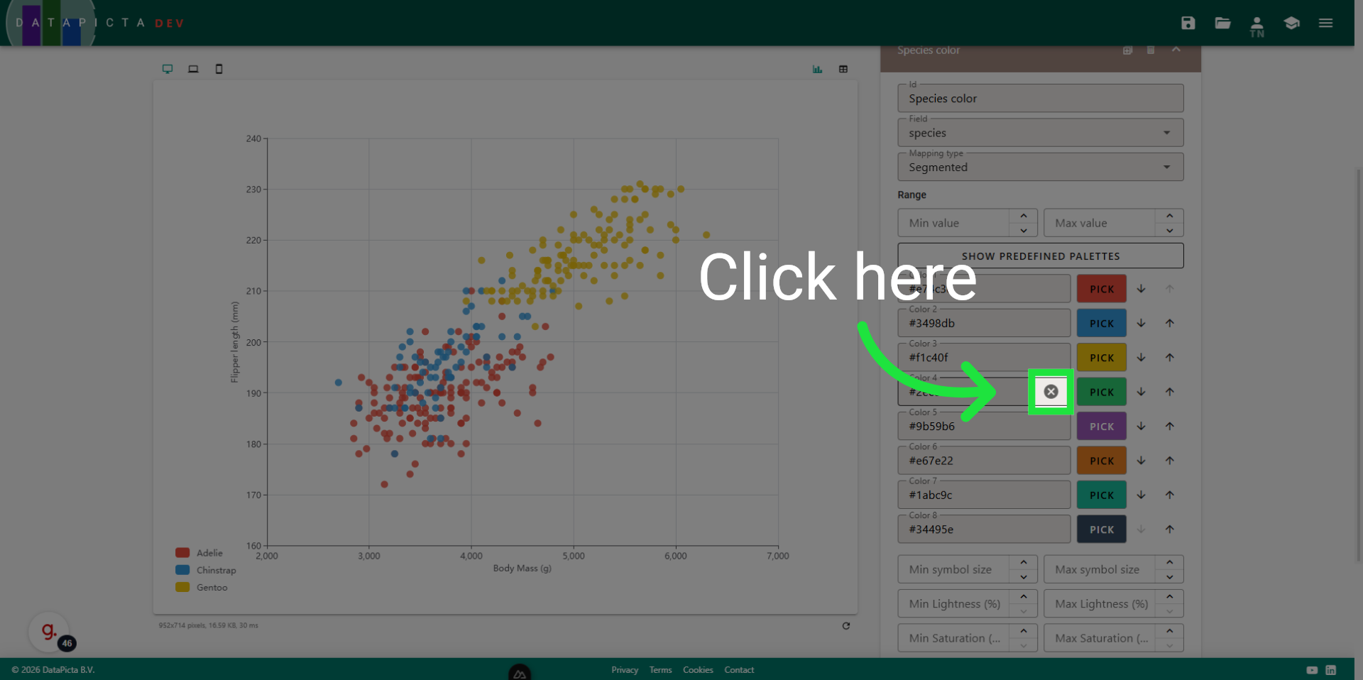
32. Remove Colors
We only need three colors, so feel free to remove any colors you don't like.
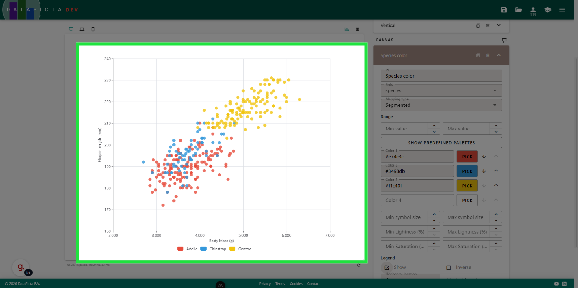
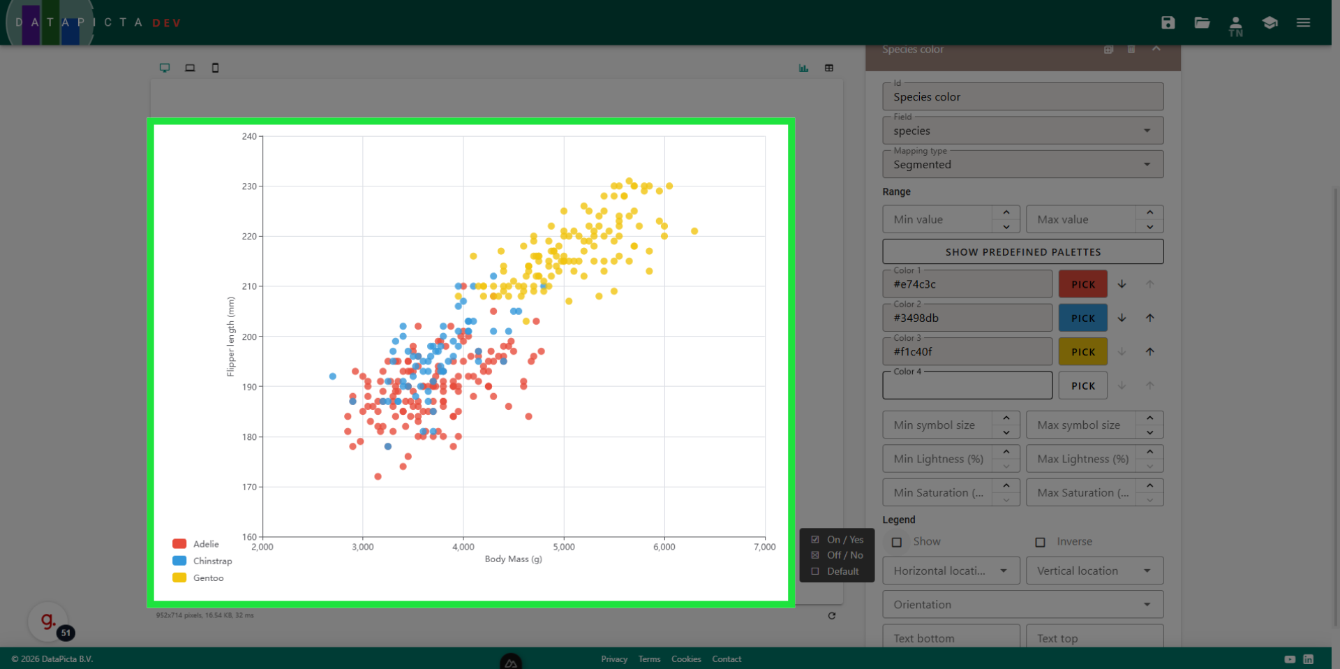
33. View Result
The selected colors are applied to the chart, and a legend for these colors is included. However, the placement of the legend could be improved.
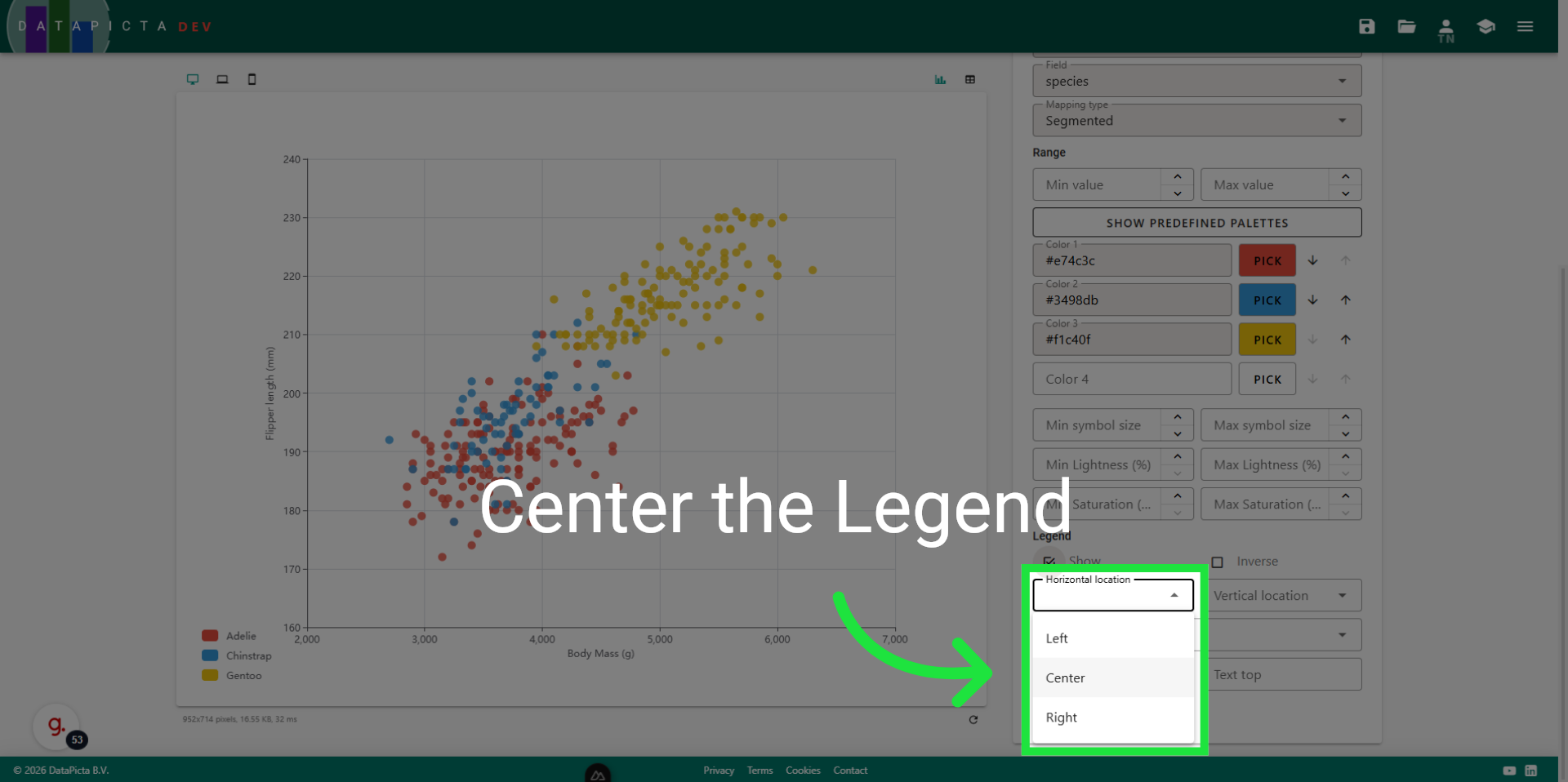
34. Set Legend Position
Now scroll down a bit and click 'Center' to center the legend horizontally within the visualization.
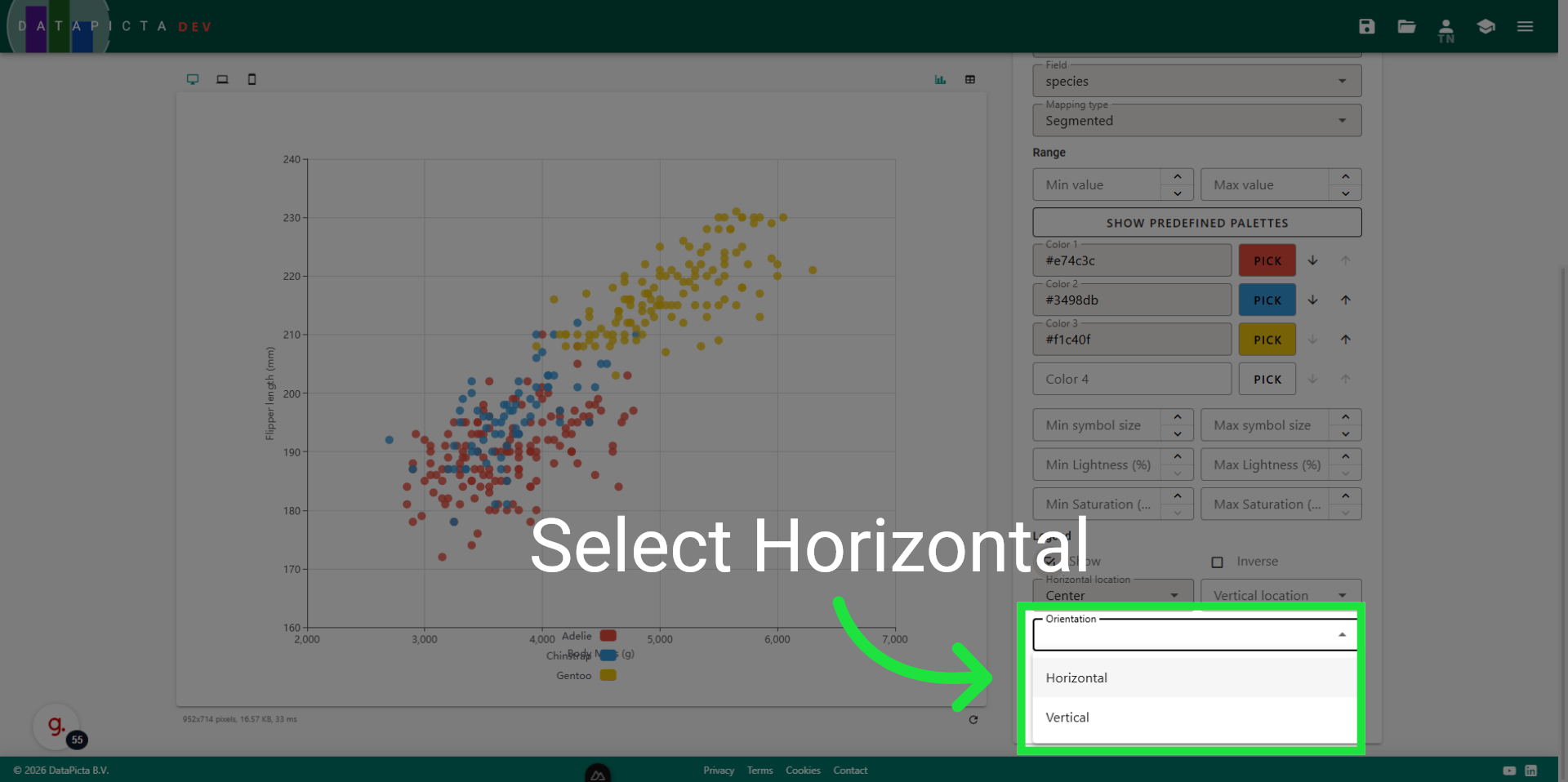
35. Set Legend Orientation
For 'Orientation', select 'Horizontal' to position the colors side by side rather than stacked on top of each other.
36. Done
You have created a vibrant scatterplot that illustrates the relationship between body mass and flipper length for three distinct species of penguins. You can now save, publish, and share your chart with your audience.